Quickly Toggle Auto-filter in MS Excel

Who knows this cool trick?

Use this shortcut to activate a filter that already exists. Excel will then display sorting and filtering options.

Steps:

1. Click in table header
2. Press Ctrl + Shift + L

Note: You must be in the cell that contains the filter (the drop-down arrow) before you use the shortcut.

Let us know what we have missed in the comments.

Delete Blank Rows Easily

Blank rows/column or blank cells in data sheets make your life painful. Here some easy way to delete blank rows/column/cells  in MS Excel.

Steps:

• Open the excel sheet where you wish to delete the empty cells
• After that select your data range
• Navigate to Home > Find & Select > Go To Special
• One Go To Special window will appear.
• Here click on Blanks radio button and click Ok
• Automatically all the blank cells will select
• Now just delete them navigating Home > Delete > Delete Sheet Rows/column/cells
• Remember, don’t click anywhere on the sheet otherwise selection will vanish
• Now all the blank rows/column/cells will be delete

Let us know what we have missed in the comments.

Sum Cells based on Background/Fill Color

As we all know that MS Excel has no formula or feature to calculate such a thing to calculate cells on their background color. Here, explained one methods that will help you to achieve this.

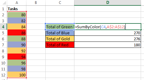
To make the task more clear let’s make a sheet as per below image.

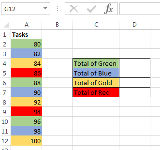
Here we don’t need the total sum of all elements but we need the sum of elements that have the same background color.

Steps: This steps is much faster and better.

For this task we can use a small UDF (User Defined Function) which will fo the trick for us. This function does not return the color name but it returns the color index which is also a unique value and can be used in our task.

• Open Worksheet
• Fill as per above background color or whatever you want
• Press Alt + F1 to open the VBA or Right click on sheet name and select View Code.
• Navigate the Insert > Module

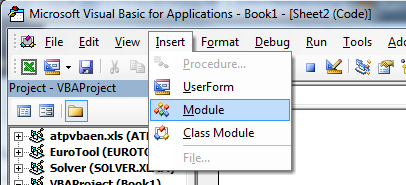
• Type the following ‘SumByColor‘ UDF in the editor

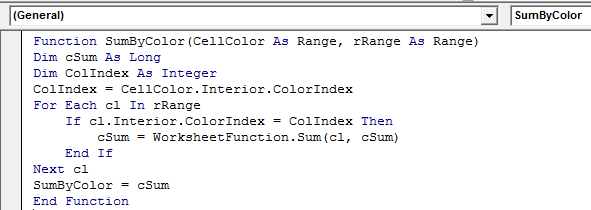
=SumByColor(Cell_with_background_color_that_you_wish_to_sum, Range_to_e_summed_up)

• Now enter the function ‘SumByColor‘ as formula
• After that, drag this formula to the whole range.

So, This is all from this topic.

Input Values Starting with 0

When an input value starts with zero, Excel will delete the zero by default. Rather than reset the Format Cells, this problem can be easily solved by adding a single quote mark ahead of the first zero, as shown.

Hide Data in Excel

Almost all user know that how to hide data by right clicking to select the Hide function, but this can be easily noticed if there is only a little bit of data.

The best and easiest way to hide data thoroughly is to use the format cells function.

Steps:

• Choose the area, you want to hide
• Go to Home > Font > Format Cells
• Click on Number Tab
• Choose Category as Custom
• Type should be ;;;
• After-that click Ok

All the values in the area will be invisible and can only be found in the preview area next to the Function button.